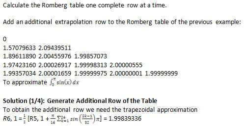
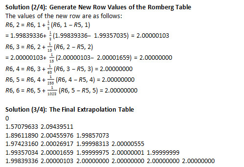
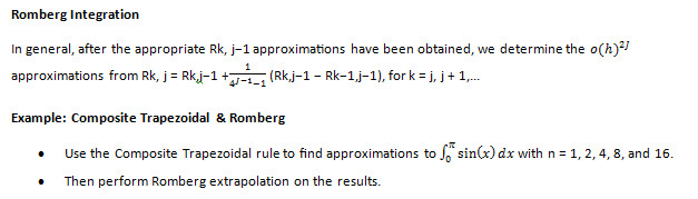
Romberg Integration
Solution (6/6): Tabulated Extrapolation Results
0
1.57079633 2.09439511
1.89611890 2.00455976 1.99857073
1.97423160 2.00026917 1.99998313 2.00000555
1.99357034 2.00001659 1.99999975 2.00000001 1.99999999
0
1.57079633 2.09439511
1.89611890 2.00455976 1.99857073
1.97423160 2.00026917 1.99998313 2.00000555
1.99357034 2.00001659 1.99999975 2.00000001 1.99999999
Romberg Integration: Recursive Calculation
- Notice that when generating the approximations for the Composite Trapezoidal Rule approximations in the last example, each consecutive approximation included all the functions evaluations from the previous approximation.
- That is, R1,1 used evaluations at 0 and π, R2,1 used these evaluations and added an evaluation at the intermediate point π/2.
- Then R3,1 used the evaluations of R2,1 and added two additional intermediate ones at π/4 and 3π/4.
- This pattern continues with R4,1 using the same evaluations as R3,1 but adding evaluations at the 4 intermediate points π/8, 3π/8, 5π/8, and 7π/8, and so on.
- This evaluation procedure for Composite Trapezoidal Rule approximations holds for an integral on any interval [a, b].
- In general, the Composite Trapezoidal Rule denoted Rk+1,1 uses the same evaluations as Rk,1 but adds evaluations at the 2k−2 intermediate points.
- Efficient calculation of these approximations can therefore be done in a recursive manner.
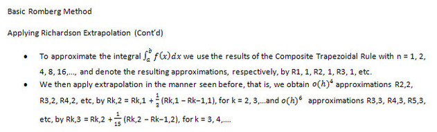
Then R1,1 = h12[f (a) + f (b)] =(b − a)2[f (a) + f (b)] and R2,1 =h2 2[f (a) + f (b) + 2f (a + h2)]
By re-expressing this result for R2,1 we can incorporate the previously determined approximation R1,1
R2,1 =(b − a) /4[ f (a) + f (b) + 2f (a +(b − a)/2)] = [R1,1+h1f (a+h2)]